A Project Based Introduction to TensorFlow.js

In this post we introduce how to use TensorFlow.js by demonstrating how it was used in the simple project Neural Titanic. In this project, we show how to visualize the evolution of the predictions of a single layer neural network as it is being trained on the tabular Titanic Dataset for the task of binary classification of passenger survival. Here’s a look at what we will produce and a link to the live demo:
This article assumes that you have a basic understanding of modern frontend JavaScript development and a general awareness of basic machine learning topics. Please let me know in the comments if you have any questions.
Outline
Neural Networks
Neural networks are finally getting their rightfully deserved day in the sun after many years of development by a rather small research community spearheaded by the likes of Geoffrey Hinton, Yoshua Bengio, Andrew Ng, and Yann LeCun. Traditional statistical models do very well on structured data,i.e. tabular data, but have notoriously struggled with unstructured data like images, audio, and natural language. Neural networks that contain many layers of neurons embody the research that is popularly called Deep Learning. The key insight and property of deep neural networks that make them suitable for modeling unstructured data is that complex data, like images, generally have many layers of unique features that are composed to produce the data. As a classic example: images have edges which form the basis for textures, textures form the basis for simple objects, simple objects form the basis for more complex objects, and so on. In deep neural networks we aim to learn these many layers of composable features. A full discussion of deep learning and neural networks is beyond the scope of this post, but here I provide links to a few talks I’ve given on the topic which contain many links to great resources.


With the dramatic increase of computing power and available data over the last few decades, neural networks became viable for solving many real world problems. Today, libraries like TensorFlow and others are accelerating the adoption of neural networks for solving more problems by making it easy for typical programmers to experiment and innovate with the technology. TensorFlow.js is not the solution for every problem, but it is another step in the direction of making neural networks more accessible to everyone. Publications like Distil have proven to me the potential of introducing neural networks to the ecosystem of the modern web for educational purposes and beyond. I hope this article inspires you to make your own neural network powered applications as well.
Project Overview
As I mentioned above, neural networks are very well suited for modeling unstructured data … why then are we applying it to the structured data of the Titanic Dataset? I admit throwing a neural network at this data is like taking a rocket ship to work in the morning, but it is hoped that seeing neural networks work on simple tabular data gives you some insight into the behavior of how neural networks learn with respect to different hyperparameters of the network — like batch size, choice of activation functions, and number of neurons. As a principle, simpler models generally perform better on simpler data due to having less capacity for overfitting/memorization. For the Titanic Dataset, and as with almost all types of tabular data, ensemble methods like boosted trees would perform better with much less hyperparameter tuning required. I mention this because upon hearing about neural networks, newcomers tend to think neural networks are the solution to every modeling problem; this is not the case and has been proven so in industry and on competitive data science platforms like Kaggle where ensemble methods reign king on structured data.
In this project we show how to visualize the evolving predictions of a single layer neural network as it is being trained on the tabular Titanic Dataset for the task of binary classification of passenger survival. The colors of each row indicate the predicted survival probability for each passenger. Red indicates a prediction that a passenger died. Green indicates a prediction that a passenger survived. The intensity of the color indicates the magnitude of the prediction probability. For example: a bright green passenger represents a strong predicted probability for survival. We also plot the loss of our objective/loss function on the left of the table with D3.js.
This post aims to show how TensorFlow.js was used in a more realistic project than what can be found in the TensorFlow.js official tutorials — which tend to avoid the complexities of creating a user interface. If you are already well versed in modern frontend JavaScript development, and exclusively use a frontend framework like React, you may be interested in a more direct tutorial that focuses mainly on TensorFlow.js.
Dataset and Modeling Overview
The Titanic Dataset is a popular dataset for introducing the basics of machine learning due to its small size and ease of interpreting what sorts of features may be helpful to predicting survival. We are tasked with predicting the survival of a passenger when given the other bits of data that describe the passenger in the table. The columns we use to predict survival are called the predictive features, traditionally labeled X. The column we are predicting is called the target label, traditionally labeled y. Here are a few rows of the dataset:
| pclass | survived | name | sex | age | sibsp | parch | ticket | fare | cabin | embarked |
|---|---|---|---|---|---|---|---|---|---|---|
| 1 | 1 | Allen, Miss. Elisabeth Walton | female | 29 | 0 | 0 | 24160 | 211.3375 | B5 | S |
| 1 | 1 | Allison, Master. Hudson Trevor | male | 0.9167 | 1 | 2 | 113781 | 151.5500 | C22 C26 | S |
| 1 | 0 | Allison, Miss. Helen Loraine | female | 2 | 1 | 2 | 113781 | 151.5500 | C22 C26 | S |
| 1 | 0 | Allison, Mr. Hudson Joshua Creighton | male | 30 | 1 | 2 | 113781 | 151.5500 | C22 C26 | S |
| 1 | 0 | Allison, Mrs. Hudson J C (Bessie Waldo Daniels) | female | 25 | 1 | 2 | 113781 | 151.5500 | C22 C26 | S |
And here are the descriptions of each field:
- Predictive Features ( X )
- pclass: the class of the passenger (1st, 2nd, 3rd )
- name: the name on the ticket, which contains the last name first
- sex: the gender of the passenger (female,male)
- age: the age of the passenger.
- sibsp: the number of siblings or spouses aboard related to the passenger.
- parch: the number of parents or children aboard related to the passenger
- ticket: the passenger’s ticket number.
- fare: the dollar amount paid for the passengers ticket.
- cabin: the cabin the passenger was assigned to.
- embarked: the port of embarkation (C = Cherbourg, Q = Queenstown, S = Southampton)
- Target Label ( y )
- survived: 1 if the passenger survived, 0 if the passenger died.
The full dataset has over 1,000 passenger rows, but for the sake of brevity let’s pretend the above table is the entirety of our dataset. We would then have the following matrix X and row vector y:
Neural networks, in a more technical sense, provide a robust framework for nonlinear function approximation. The problem of predicting the survival of the passengers y given the passenger features X can be formulated as finding a function such that:
In the case of neural networks we learn this function and the process of learning it is called training. In all non-trivial problems we can only approximate this function and in practice we never actually want to find the precise function that satisfies this equation; because if we do, we are most likely to have found a function that memorizes the dataset and does not represent a function that will accurately predict y given X on data it has not trained on. The ability to make good predictions on data we have not trained on is called generalization and is largely related to the bias-variance problem. Being a deep learning practitioner requires you to construct neural network architectures that approximate these types of functions while also generalizing well to unseen data.
Project Setup
We use the webpack bundler to bundle our JavaScript source code for distribution and the webpack dev server for development so that we do not have to manually bundle our code every time we make a change in development.

./data/ : we have a csv containing the titanic dataset.
./dist/: this is the distribution folder that will be the target of our webpack bundle.
./src/: here we have the JavaScript and CSS source code.
./static/ : here are the static assets, which in this case is just our logo and favicon.
This repo is a npm package defined by the package.json file and we store our scripts (build,dev) for working with the project and a list relevant dependencies there. We also have a webpack.config.js file for configuring how webpack should work on this project.
To get started with this project, do the following:
- Install Node.js.
- Clone or download this repo.
- Open a terminal and cd into your copy of the repo.
- In your terminal type: npm install
- Launch the dev server by typing: npm run dev
- Click on the url shown in the terminal or enter http://localhost:8080/ in your web browser.
On step #4 you use npm to install the project dependencies listed in package.json. On step #5 you launch the dev server which displays a URL you should click in step #6. At this point, whenever you save a modification to the source code it will prompt the development server to refresh the web page you have open and will display your changes immediately.
When you are ready to bundle your code for serving, simply run npm run build and it will produce the files you can put on your web server in the ./dist/ folder.
Now that you have the code and ability to make changes and quickly see the results, let’s look at the important pieces of code.
The Code
Here we provide extended documentation and commentary for the critical code of the project. If you already know modern fronted JavaScript development well,you may want to skip to modeling.js and preprocessing.js. I skip certain parts of the code that are dry and would be tiresome to explain. Clone the repo for this project to get all the code.
index.html
Here we define the HTML template for the application. It has many extraneous things related to the description section, but I will point out a few key parts. There are a few main containers in the HTML template we modify with our JavaScript code:
- #trainingCurves: the loss function svg container.
- #modelParameters: the container for the model parameter input elements.
- #trainBttnContainer: the container for the start/stop training button.
- #tableControls: container for the sorting selection menu.
- #dat: container for the table data.
At the bottom of the file you will notice the following:
<script src="bundle.js"></script>This includes the JavaScript and CSS code bundled by webpack.
index.js
This is our application’s entry point. The code in this file kicks off the rest of the application.
import * as d3 from 'd3';
import 'bootstrap';
import './scss/app.scss';
import {createTrainBttn,makeTable,createSortByMenu,attachChangeParameterHandler} from './ui';
import {startTraining} from './events';
We use ES6 import statements to import other JavaScript modules and the CSS which is also bundled with the rest of our code. Bundling CSS with JavaScript is not particularly best practice, but will suit our purpose. See this link for more information on splitting your dependencies.
After the these imports we have inside the main function the following code:
d3.dsv(",", "data/titanicData.csv", function(d) {
    return {d}
})
.then(function(data) {
    createTrainBttn("train",data);
    createSortByMenu(data);
    startTraining(data);
    makeTable(data);
    attachChangeParameterHandler();
});
Here we use D3.js, as imported above, to load a CSV file titanicData.csv containing the titanic dataset. After the CSV is loaded, it triggers the attached then function which: instantiates parts of the user interface ( createTrainBttn, createSortByMenu, attachChangeParameterHandler), initiates the training ( startTraining ), and displays the data in a table (makeTable). As you can see, each function is passed a reference to the loaded data. I have tried to make this particular project as functional as possible; which means I typically try to avoid global variables and reconstruct elements of the UI when they change. This was a design decision I made to reduce the need for a state management system, but would undoubtedly become cumbersome in a more complex project.
ui.js
This module is responsible for handling the user interface functionality. It is rather primitive with respect to some other applications which use frameworks like React, but for this reason, it is hoped that it has less intellectual overhead and is easier for newcomers to understand.
const svg = d3.select("#trainingCurves").select("svg");
const margin = {top: 20, right: 20, bottom: 20, left: 20};
const width  = +svg.attr("width") - margin.left - margin.right;
const height = +svg.attr("height") - margin.top - margin.bottom;
Here we define constants defined within this module’s scope for the properties of the svg canvas we use to plot the loss function. Only code in this module can access these variables because we do not use the keyword export.
export function createTrainBttn(state,titanicData){
    // Select the button.
    var bttn = d3.select("#trainBttnContainer").select("button");

    // If there is no button, create one.
    if(bttn.empty()){
        bttn = d3.select("#trainBttnContainer").append("button");
    }

    // Change the button state based on the input argument state.
    if(state == "train"){
        // Make the button the start training button.
        bttn
        .attr("id","startBttn").attr("class","btn btn-success btn-lg")
        .on("click",()=>startTraining(titanicData)).text("Start Training");
    }else{
        // Make the button the stop training button.
        bttn
        .attr("id","startBttn").attr("class","btn btn-danger btn-lg")
        .on("click",()=>stopTraining(titanicData)).text("Stop Training");
    }
}
Here we handle the logic for changing the state of the start/stop training button. The only seemingly odd part here is that when we attach the event handler with the on function, we create an ES6 lambda function. This is done so we can pass along the data variable needed for those functions. This is another design choice made to reduce the need for global variables.
export function blankTrainingPlot(){
    d3.select("#trainingCurves").select("svg").selectAll("*").remove();

    d3.select("#trainingCurves").select("svg").append("text")
    .style("font","bold 30px sans-serif").attr("x","48").attr("y","160")
    .attr("fill","rgba(57, 57, 121, 0.692)").text("Start Training");
}
This function clears the loss function plot and draws the text “Start Training”.
function predToColor(pred){
    var color = "0,0,0";
    var alpha = 0.0;

    if(pred < 0.5){
        // More probable to die.
        color = "255,0,0";
        alpha=(0.5-pred)*2;
    }else{
        // More probable to survive.
        color = "0,255,0";
        alpha=(pred-0.5)*2;
    }

    return "rgba("+color+","+alpha+")";
}
This function produces the appropriate color for a prediction that we use in the next section to color the table rows. We will see later that our neural network predicts a value [0,1]. The closer this value is to 0, the more the network believes the passenger has died. Likewise, the closer the value is to 1, the more the network believes the passenger has survived. A predicted value of 0.5 represents maximum uncertainty. Thus, if the predicted value is less that this threshold of 0.5, we output a red cell with an alpha ( transparency level ) that is proportional to how strong the network predicts death (i.e. dark red represents a strong prediction of passenger death ). The same logic is applied to the survival case.
What does predToColor(0.1) produce? 0.1 < 0.5 so we will be producing a red color. What about the alpha?
Thus we produce a very strong red color: predToColor(0.1) = “rgba(255,0,0,0.8)”. This color would then be used to color the corresponding row in the table corresponding to passenger the neural network made a prediction on.
Question for you: Why do we process the alpha values in this way? Why don’t we simply use the predicted value as the alpha value?
export function updatePredictions(predictions){
    const predColor = _.map(predictions,predToColor);
    d3.select("#dat").select("table").select("tbody")
    .selectAll("tr").data(predColor).style("background-color",(x)=>x);
}
Here we actually use predToColor defined in the previous snippet to color the table rows. The input to this function is an array of predictions for all the rows in the table. We map predToColor over all these predictions and get an array of corresponding color values. We then use d3 to iterate over the table and update the background-color of each cell with the new prediction colors. Here you can see the elegance of d3’s data binding functionality.
export async function plotLoss(lossData,accuracy){
    // Modified from: https://bl.ocks.org/mbostock/3883245
    var g = svg.select("g");
    var lossText = svg.select("text");
    var y = d3.scaleLinear().rangeRound([height, 0]);
    var x = d3.scaleLinear().rangeRound([0, width/lossData.length]);
    var data = _.zip(_.range(lossData.length),lossData);
    var line = d3.line()
    .x(function(d) { return x(d[0]); })
    .y(function(d) { return y(d[1]); });

    g.select("path")
        .datum(data)
        .attr("fill", "none")
        .attr("stroke", "steelblue")
        .attr("stroke-linejoin", "round")
        .attr("stroke-linecap", "round")
        .attr("stroke-width",3)
        .attr("d", line);

    lossText.text("Loss: "+lossData[lossData.length-1].toFixed(3)+" | Accuracy: "+(accuracy*100).toFixed(2)+"%");
}
This is the D3 code that plots the loss curve. It is called from the training process which we will look at shortly. It is passed an array of loss values of the neural network over the training epochs and the current epoch accuracy. I cannot go into the full details of D3 in this post. Please see the introduction to D3.js if you’d like to understand this code more.
export function makeTable(data){
    d3.select("#dat").selectAll("*").remove();

    // Create Table
    var table = d3.select("#dat").append("table").attr("class","table");

    // Create Table Header
    table.append("thead").append("tr")
    .selectAll('th').data(data.columns).enter()
    .append("th").text(function (column) { return column; });

    // Populate Table
    table.append("tbody").selectAll("tr").data(data).enter().append("tr")
    .selectAll("td").data(function (d){return Object.values(d.d);}).enter().append("td")
    .text(function(d){return d}).exit();
}
Another bit of d3 code that creates the HTML table from the csv data loaded above in the index.js snippet.
preprocessing.js
function prepTitanicRow(row){
    var sex = [0,0];
    var embarked = [0,0,0];
    var pclass = [0,0,0];
    var age = row["age"];
    var sibsp = row["sibsp"];
    var parch = row["parch"];
    var fare = row["fare"];

    // Process Categorical Variables
    if(row["sex"] == "male"){
        sex = [0,1];
    }else if(row["sex"] == "female"){
        sex = [1,0];
    }

    if(row["embarked"] == "S"){
        embarked = [0,0,1];
    }
    else if(row["embarked"] == "C"){
        embarked = [0,1,0];
    }
    else if(row["embarked"] == "Q"){
        embarked = [1,0,0];
    }

    if(row["Pclass"] == 1){
        pclass   = [0,0,1];
    }
    else if(row["Pclass"] == 2){
        pclass   = [0,1,0];
    }
    else if(row["Pclass"] == 3){
        pclass   = [1,0,0];
    }

    // Process Quantitative Variables
    if(parseFloat(age) == NaN){
        age = 0;
    }
    if(parseFloat(sibsp) == NaN){
        sibsp = 0;
    }
    if(parseFloat(parch) == NaN){
        parch = 0;
    }
    if(parseFloat(fare) == NaN){
        fare = 0;
    }

    return pclass.concat(sex).concat([age,sibsp,parch,fare]).concat(embarked);
}
This is the code for preprocessing each row of the titanic dataset; which simply consists of turning categorical variables into a one-hot representation and setting NaN values to 0. There are more elegant means of preprocessing, including methods like infilling NaNs, and you may notice that we omit several fields in the data that would be harder to process such as name. This was done to simplify the code, as this project was originally created from some teaching materials I prepared. Feel free to figure out how you may want to include the omitted features for better predictions.
export function titanicPreprocess(data){
    const X = _.map(_.map(data,(x)=>x.d),prepTitanicRow);
    const y = _.map(data,(x)=>x.d["survived"]);
    return [X,y];
}
Here we map the preprocessing function prepTitanicRow over each row of the data. The output of this function is the feature matrix X and target vector y as described above.
Now that we have described the main parts of the boring side of the application, let’s actually look at the neural network part.
modeling.js
export function createModel(actFn,nNeurons){
    const initStrat = "leCunNormal";
    const model = tf.sequential();
    model.add(tf.layers.dense({units:nNeurons,activation:actFn,kernelInitializer:initStrat,inputShape:[12]}));
    model.add(tf.layers.dense({units:1,activation:"sigmoid",kernelInitializer:initStrat}));
    model.compile({optimizer: "adam", loss: tf.losses.logLoss});
    return model;
}
We have finally come to the point where we make our little single layer neural network. The creation of the network is parameterized by the variables actFn and nNeurons set by the user in the user interface. You may notice that the number of inputs to our network outnumber the number of features we actually have. This is because we expand the dimensionality of the feature space in the preprocessing step above; i.e. instead of having a single input for the port of embarkation, we now have a one-hot vector of length 3. Will will go through this code line by line, but before we do, here’s a visual of what the network looks like:
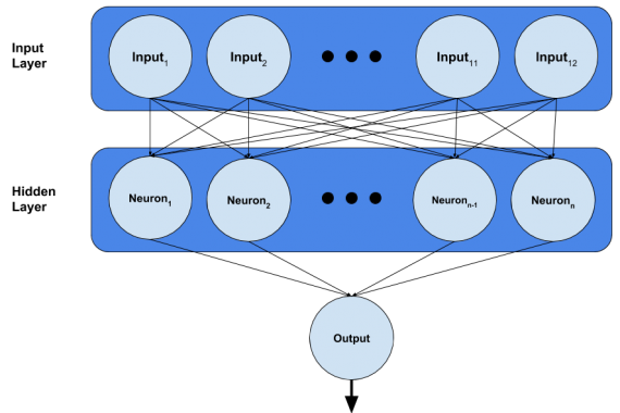
const initStrat = "leCunNormal";The connections, called edges, you see in the network are weighted, and adjusting these weights is what we do when we train the network. Since our training is iterative, we must have some initial state for the weights. The scheme we use for setting the initial state of the weights is called the initialization strategy. Typically you could avoid explicitly stating an initialization strategy because the default initialization strategy used by TensorFlow of sampling the initial weights from a uniform distribution works well enough in many cases, but for many other cases the initial state of these weights highly influences the performance of the network. Since we have a very small dataset, the performance of our network is highly dependent upon the initial state of the weights. Due to this, I have chosen an initialization strategy that produces more consistent results in this case.
const model = tf.sequential();The sequential model object is what we will use to build our model. A sequential model simply means that when we add layers to the model, they will be stacked sequentially like shown in the network diagram above.
model.add(tf.layers.dense({units:nNeurons,activation:actFn,kernelInitializer:initStrat,inputShape:[12]}));Here we implicitly add the input layer ( of size 12 ) and add the hidden densely connected layer to the network. A densely connected layer simply means that every neuron in the layer will be connected to every neuron in the layer before it. In our case, the hidden layer is attached to an input layer, so every neuron in the hidden layer is connected to every input in the input layer. These inputs are represented in the diagram above as circles like the neurons, but it is important to note that these are inputs not neurons; however, they are still connected to the elements in the hidden layer as two layers of neurons would be connected.
The dense layer takes in a dictionary of arguments defining the layer. There are many such arguments,but we only need to provide the arguments which we require to be different from the default arguments:
- units: The number of neurons. As we showed above, this parameter is adjustable by the user from the user interface.
- activation: The activation function for each of the neurons in this layer. Again, this is something that is set by the user in the ui. A full discussion on activation functions is outside the scope of this piece, but I encourage you to play with the demo and see how changing the activation function changes the predictions before delving into the formal theory of these things.
- kernelInitializer: We set this above and discussed its purpose.
- inputShape: This is the size of the implicitly created input layer. In our case, we have an input layer of 12 units.
model.add(tf.layers.dense({units:1,activation:"sigmoid",kernelInitializer:initStrat}));This is the last layer of our network, which is simply a single output neuron that is densely connected to the hidden layer. We use a sigmoid function as the activation for this unit because we want our network to predict a probability for passenger survival [0,1] and this is precisely the range of the sigmoid function. There are other functions with this range, of course, and a natural question you may have is: “Why use this function over others for predicting a probability?” While an answer to this question is beyond the scope of this piece, I will say to those inquiring minds that the use of the sigmoid function comes from the heritage of logistic regression.
model.compile({optimizer: "adam", loss: tf.losses.logLoss});In the steps prior, we have setup the network architecture, but have not actually made the model. When we compile a neural network in TensorFlow, we actually produce the network. You will typically supply two arguments to the network compiler:
- optimizer: This is the optimization algorithm we use during training. At the risk of bringing the flames of the ML community to my rear, I will say that if you are a novice, just use Adam. It is very important to understand [how these optimizers work]((http://www.deeplearningbook.org/contents/optimization.html) when you are doing machine learning research because when certain problems occur you must be able to reason about all the parts of the network and training process, but for a newcomer, Adam will work consistently enough for you not to worry until you really get into hard problems.
- loss: The loss function demands more of your attention, as different modeling problems require different loss functions. A loss function tells us how to measure the discrepancy between our model’s predictions and actual target values. We use this measure of error to train our network in conjunction with the optimizer and back-propagation. In the case of modeling probability, you will typically use a variant of cross-entropy loss, as is log loss.
After having dealt with the complexities of the user interface and creating the model, what’s left? We now must tackle the actual training of the model.
export async function trainModel(data,trainState){
    // Disable Form Inputs
    d3.select("#modelParameters").selectAll(".form-control").attr('disabled', 'disabled');
    d3.select("#tableControls").selectAll(".form-control").attr('disabled', 'disabled');

    // Create Model
    const model = createModel(d3.select("#activationFunction").property("value"),
                              parseInt(d3.select("#nNeurons").property("value")));

    // Preprocess Data
    const cleanedData = titanicPreprocess(data);
    const X = cleanedData[0];
    const y = cleanedData[1];

    // Train Model
    const lossValues = [];
    var lastBatchLoss = null;

    // Get Hyperparameter Settings
    const epochs    = d3.select("#epochs").property("value");
    const batchSize = d3.select("#batchSize").property("value")

    // Init training curve plotting.
    initPlot();

    for(let epoch = 0; epoch < epochs && trainState.s; epoch++ ){
        try{
            var i = 0;
            while(trainState.s){
                // Select Batch
                const [xs,ys] = tf.tidy(() => {
                    const xs = tf.tensor(X.slice(i*batchSize,(i+1)*batchSize))
                    const ys = tf.tensor(y.slice(i*batchSize,(i+1)*batchSize))
                    return [xs,ys];
                });

                const history = await model.fit(xs, ys, {batchSize: batchSize, epochs: 1});
                lastBatchLoss = history.history.loss[0];

                tf.dispose([xs, ys]);
                await tf.nextFrame();
                i++;
            }
        }catch(err){
            // End of epoch.
            //console.log("Epoch "+epoch+"/"+epochs+" ended.");
            const xs = tf.tensor(X);
            const pred = model.predict(xs).dataSync();
            updatePredictions(pred);

            const accuracy = _.sum(_.map(_.zip(pred,y),(x)=> (Math.round(x[0]) == x[1]) ? 1 : 0))/pred.length;

            lossValues.push(lastBatchLoss);
            plotLoss(lossValues,accuracy);

        }
    }
    trainState.s = true;
    createTrainBttn("train",data);
    console.log("End Training");

    // Enable Form Controls
    d3.select("#modelParameters").selectAll(".form-control").attr('disabled', null);
    d3.select("#tableControls").selectAll(".form-control").attr('disabled', null);

}
Before getting into this, I will define some terms used:
- Epoch: training a model on one the entirety of the dataset once. Those coming from non-stochastic modeling backgrounds may find the process of stochastic optimization very strange at first, but the idea is quite natural to us. When you first study a subject, do you understand it completely without iteration? Of course not; we must constantly work at improving our understanding. Even though all the subject material may be presented at once, we need to go over it multiple times to understand it.
- Mini-Batch: a subset of the full training data. During each epoch, we split the training data into smaller batches to train on. To continue the analogy started above, when you learn something like mathematics, you approximate a general understanding of mathematics by studying different parts. It would be impossible for us to learn all of mathematics at once, given our limited capacity.
Here what’s happening at a high level in this function:
- Create the neural network.
- Preprocess the data.
- Epoch Loop: Train network for the number of epochs set by the user.
- Mini-Batch Loop: While we still have data to train on in the current epoch and the user hasn’t stopped the training.
- Train the model on a mini-batch.
- End of epoch: Now that we have further trained the model, we make new predictions on the data and update the predictions using the user interface function updatePredictions.
- Mini-Batch Loop: While we still have data to train on in the current epoch and the user hasn’t stopped the training.
Going over this code line by line would be tedious for both you and I, so I will address some key points and questions that will likely puzzle you and puzzled me.
What’s with “async” and “await”?
This is the part of ES6 which allows us to define asynchronous functions. We use await when training the model because that too is an asynchronous function and would like to wait for it to finish training before moving onto the next epoch.
tf.tidy and tf.dispose?
These functions are involved with the garbage collection of the tensors created. You should read about the core concepts in TensorFlow.js for more detail.
await tf.nextFrame();
Without this bit, the training of the model would freeze your browser. This function is sparsely documented and is most likely a product of TensorFlow.js being in early development. I would expect future versions to mitigate the need to explicitly call this function. Figuring out where to use this function caused me the most frustration in this project.
tf.tensor() and dataSync();
Because our data is stored in standard JavaScript arrays, we need to convert them to TensorFlow’s tensor format with tf.tensor(). When we want to go the other way, from tensor to JavaScript array, we call the dataSync() function of a tensor.
Summary
In this article we discussed a complete modern JavaScript project that uses TensorFlow.js to visualize the evolving predictions of a single layer neural network as it is being trained on the tabular Titanic Dataset for the task of binary classification of passenger survival. We hope that this will help you understand how you can use TensorFlow.js in your projects. If this is your first experience with TensorFlow or neural networks, please consider checking out the following resources for a more comprehensive coverage of the essentials: